Introduction
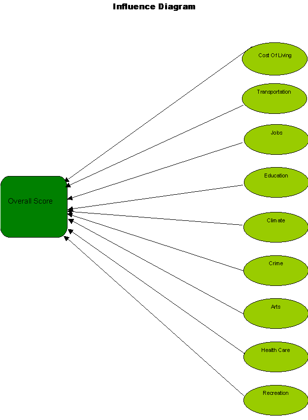
The data collected from the book Places Rated Almanac rated 325 metro areas based on various factors such as
1) Transportation
2) Jobs
3) Education
4) Climate
5) Crime
6) Arts
7) Health Care
8) Recreation
Based on the above factors an overall score has been assigned to each metro area. Our objective is to explore the potential relationship between these factors and the Overall score.

Analysis
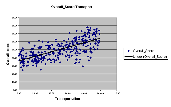
The factors listed above can be considered as potential explanatory or independent variables and the score as a dependent variable. The relationships between each of the listed explanatory variables and the score are shown below.
|
|
Transportation |
Jobs |
Education |
Climate |
Crime |
Arts |
Health_Care |
Recreation |
Overall_Score |
|
Transportation |
1.0000 |
|
|
|
|
|
|
|
|
|
Jobs |
0.3846 |
1.0000 |
|
|
|
|
|
|
|
|
Education |
0.6071 |
0.3847 |
1.0000 |
|
|
|
|
|
|
|
Climate |
-0.0911 |
0.3302 |
-0.1035 |
1.0000 |
|
|
|
|
|
|
Crime |
-0.1337 |
-0.2691 |
-0.0563 |
-0.4420 |
1.0000 |
|
|
|
|
|
Arts |
0.7135 |
0.4392 |
0.6523 |
-0.1025 |
-0.1352 |
1.0000 |
|
|
|
|
Health_Care |
0.3569 |
0.3233 |
0.5089 |
-0.0879 |
-0.1141 |
0.5655 |
1.0000 |
|
|
|
Recreation |
0.5052 |
0.5489 |
0.4798 |
0.2456 |
-0.2266 |
0.6077 |
0.3516 |
1.0000 |
|
|
Overall_Score |
0.6966 |
0.6747 |
0.7663 |
0.0963 |
-0.0416 |
0.8002 |
0.6799 |
0.7456 |
1.0000 |
From the correlation table we can see that
the seven highlighted
factors have a higher correlation with Overall score. In other words, we can
expect a considerable change in the Overall score when either one of these
seven variables varies.

|
Regression
output for Overall_Score versus Transportation |
||||
|
|
|
|
|
|
|
Regression
Statistics |
|
|
|
|
|
Multiple R |
0.69657257 |
|
|
|
|
R Square |
0.48521335 |
|
|
|
|
Adjusted R Square |
0.48361958 |
|
|
|
|
Standard Error |
8.44200483 |
|
|
|
|
|
|
|
|
|
|
|
Coefficients |
Standard Error |
t Stat |
P-value |
|
Intercept |
36.06417 |
1.206930168 |
49.08786 |
8E-152 |
|
Transportation |
0.28127267 |
0.02012861 |
-8.8473 |
5.98E-17 |
Predicted Overall_score = 36.06 +0.28( Transportation)
Thus, we could draw
scatter plots of each of independent
variables and the dependent
variable and also carry
out regression analysis – by including one independent variable at a time and
arrive at our final model. Instead,
since there are a number of explanatory variables we could arrive at our final
model by conducting a Multiple Regression Analysis.
Multiple regression
|
|
|
|
|
|
|
|
|||||||||||||||||||||||||||||||||||||||||||||||||||||||||||||||||||||||||||||||||||||||||||||||||||||||||||||||||||||||||||||||||||||||||||||||||||||||||||||||||||||||||||||||||||||||||||||||||||||||||||||||||||||||||||||||||
We can now write
the regression output from the above results as
Predicted
Overall_Score = 12.88 +0.068(Transportation)+ 0.125(Jobs) + 0.100(Education) +
0.07(Climate)+ 0.09(Crime)+0.07(Arts) +0.12(Health Care)+ 0.092 (Recreation)
From the above results, it can be observed that p-
values for all the coefficients are zero which means that all the explanatory
variables are significant. R Square value is 96% meaning that the set of explanatory variables has
done a good job of explaining the
variance in Overall Score.
Implementation
& Use :
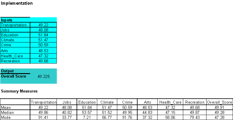
Now that we have arrived at the equations that help
us to predict overall score using the values of different variables, we can use this information to predict the
Overall_Score for any other metro area not listed in the data table provided we
have sufficient information about all the variables.
Also, any city’s
administration can use this analysis and find out the factors that highly
affect the Overall_score and take remedial action. For example, if for some city “Jobs” has a detrimental effect on the Overall_Score then the
administration can take steps to improve on this so as to make the city a more
attractive option.
