Project 3 B -Part 1

Simulations allow us to build the uncertainty ( present in most business problems) explicitly into spread sheet models. The spread sheet model will contain some cells which have random values with given probability distributions. Every time the spread sheet recalculates, these random values change, which causes the “bottom line “ output cells to change as well. The key is to run the simulations a number of times while keeping track of various outputs. This will help us to figure out the most likely outputs and see the best & worst case scenarios.

Monte Carlo simulation (MCS) is a methodology to assess risk in outcome /outcomes. MCS incorporates both sensitivity and scenario analysis and allows us to simulate thousands of scenarios within seconds while providing us with a range of values for decision making.

Sensitivity analysis allows the user to change only one variable at a time which is a serious limitation while performing complex simulations. Both sensitivity and scenario analysis are time consuming and slow processes especially for complex simulations.

Whereas MCS provides us with automated scenario analysis capability. MCS combined with a good DSS will help us to improve our decision making process and make it more reliable.

There are various steps involved in performing a MCS :

1. Define uncertain inputs using various probability distributions. A distribution is typically chosen on the basis of historical data of the inputs.
2. Select a value of randomly from each input distribution.
3. Compute outcomes
4. Repeat the steps 2 & 3 a number of times.
5. Summarize results and assess risk

Complex spread sheet simulations can be easily performed with spreadsheet add-ins like @Risk. @ Risk uses Monte Carlo simulations to perform risk analysis. Using the example below we can demonstrate the procedure used by @risk to perform MCS.

The ABC company wants to develop a projected monthly statement for the coming year. However, ABC recognizes that many of the inputs are at best educated guesses.

We can therefore, use @Risk to indicate how important bottom line figures, are to inputs.

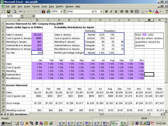
1. To begin with, we have to model the uncertainty of various inputs using various probability distributions. Therefore, we make the following assumptions.

Probability distributions for inputs
	Distribution	Parameters
Sales in January	Normal	2225	150
Cost of goods in January	Uniform	870	910
Marketing in January	Triangular	90	93	96
Administrative in January	Triangular	75	78	81
Miscellaneous in January	Triangular	23	24	25
Monthly percentage changes	Normal	1.5%	1.0%

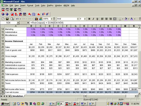
The screen shot below shows ABC’s projected income statement for the coming year.

In this example there are six uncertain inputs. The cells B12 to L16 contain probability distributions ( This is achieved by using Risk’s several functions such as RISKNORMAL, RISKUNIFORM etc.).These functions determine the generated inputs. For example, January sales has a normal distribution with a mean of 2225 and a standard deviation of 150. Therefore its function is RISKNORMAL and inputs for sales will be based on this function

2. Specifying outputs:

3. Simulation : Select the number of iterations that you would like to carry out and run it.

4. Summarize the results.

Thus MCS allows us to determine the probability distributions of our outputs using the probability distributions of our uncertain inputs. The simulation gives detailed summary statistics about all of the selected outputs. It also helps us to see the most probable outcomes given the uncertainty in our inputs. Thus, making a complex process much more easier to understand and comprehend.

Results

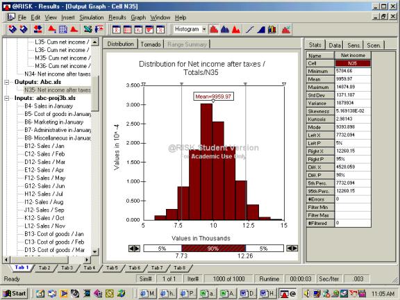
Results were viewed as summary statistics and in graphical form. From the distribution of net income after taxes we can say with 90% confidence, net income after taxes will fall somewhere between $7,730000 – $12,260,000 for the year .Total Net Income had a minimum of $5784, a mean (expected value) of $9,960, and a maximum of $14,874. This information was available for every month and more detailed summary information was available (i.e. standard deviation, variance, mode, percentile, etc.).

Our example shows that ABC will most likely generate $9,960 in net income for this year with a standard deviation of $1,300. A graphical analysis shows that our possible outcomes have a normal distribution (probability of 95% that our net income will be within 2 standard deviations from our mean/expected value).