Project 2: Exploratory Data Analysis
OBJECTIVE
In this project, we are trying to forecast a firm’s demand for its product in order to plan its future operations. In the past, the firm has used predictions of Total Industry Demand (TID) and it’s Market Share (MS) to forecast the demand for its products. FD= TID x MS. The predictions made using this method have not been very reliable due to the subjective nature of estimates. Therefore, the firm has decided to use regression analysis in order to ensure more reliable forecasts. There is enough data to perform regression analysis on TID and Relative Demand (RD) to help forecast the Firm’s Demand (FD). The model that will be used to determine the firm’s demand is (FD = TID x RD/N) Firm Demand = Total Industry Demand times Relative Demand divided by the Number of firms. TID is a function of three predictor variables, the time or quarter#, average price and average advertising. RD is a function of the following: PREL (Firm’s Price divided by Industry’s Average Price), AREL (Firm’s Advertising divided by the Industry’s Average Advertising) and RD1 (last quarter’s RD) a measure of brand loyalty.
VARIABLES
TID
Variables
¨ TID is the dependent variable.
¨ Quarter #, Avg. Price and Avg. Advertising are the independent variables.
Time series plots of TID Variables
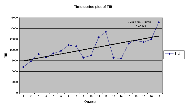
¨ The graph indicates that TID tends to increase over time. We can also see a slight cyclical trend.
¨ R Squared value suggests that the variance of the independent variable
(Quarter #) explains 48% of the variance in the dependent variable TID
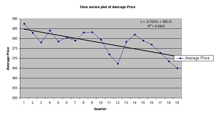
¨ Price tends to decrease over time and from the trend line equation we can see that only 49% of the variability of Average Price can be explained.
¨
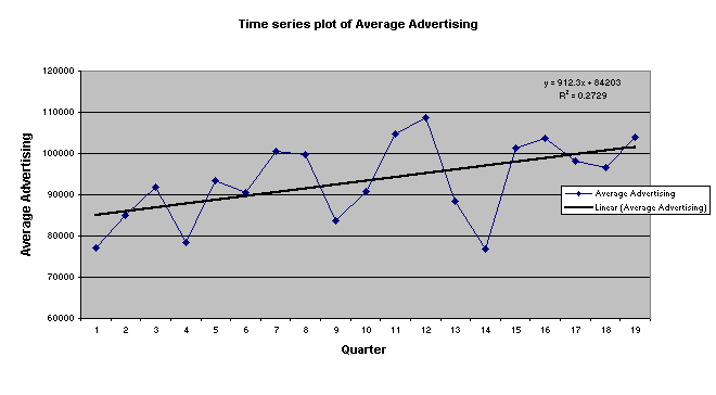
Advertising also tends to increase over time and from
the trend equation we can see that only 27% of the variability of the average
advertising has been explained.
Analyzing relationships between dependent &
independent variables
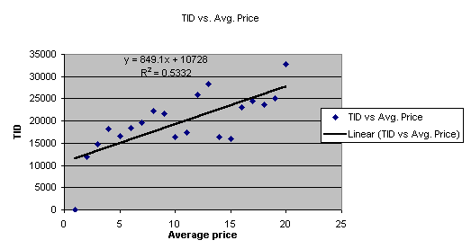
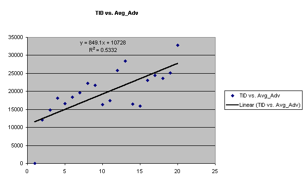
¨ There is evidence of a linear relationship between these 2 variables, the data forms an upward sloping line.
¨ From the R2 value we can see that 53% of the variability in TID has been explained.
¨ There is also a linear relationship between these 2 variables, although this one is a downward sloping line indicating an inverse relationship and economic law that states that increasing the price leads to decrease in demand.
¨ R2 value suggests that 53% of the variability of TID has been explained.
¨ These 2 scatter plots suggest that Avg. Price and Avg. Advertising are stronger measures to forecast demand than the variable “Quarter #”.
The Correlation matrix below shows the relationship
between all variables.
|
|
Quarter |
Avg_Price |
Avg_Adv |
TID |
|
Quarter |
1 |
|
|
|
|
Avg_Price |
-0.703 |
1 |
|
|
|
Avg_Adv |
0.522361 |
-0.74883 |
1 |
|
|
TID |
0.694657 |
-0.88869 |
0.882219 |
1 |
¨ From the Correlation matrix we can see that TID has high correlation with all of the variables.
¨ Correlation between independent variables should be low, but in this case all the independent variables are highly correlated. This indicates that we may have to drop one or more of the explanatory variables.
RD Variables
¨ RD is the dependent variable; it is computed by dividing Firm Demand by Industry’s Average Demand. RD measures competitive strength.
¨ PREL measures Relative Price and is an independent variable. PREL is computed by dividing the firms’ price by the Industry’s Average Price.
¨ AREL measures Relative Advertising and is an independent variable. AREL is computed by dividing the firms’ advertising by the Industry’s Average Advertising.
¨ RD1 measures brand loyalty and is also an independent variable.
¨
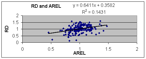
There is an inverse linear relationship between RD and PREL.
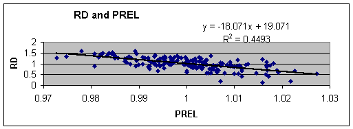
¨ The linear relationship below between RD and AREL is not very strong. The R Squared value is low.
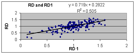
¨ The Scatter plot below indicates a fairly strong linear relationship between RD and RD1
Mathematical Modeling
TID Model 1
SUMMARY OUTPUT |
|
|
|
|
|
|
|
|
|
|
|
|
|
|
|
|
|
|
|
Regression Statistics |
|
|
|
|
|
|
|
|
|
Multiple
R |
0.69465741 |
|
|
|
|
|
|
|
|
R Square |
0.48254892 |
|
|
|
|
|
|
|
|
Adjusted
R Square |
0.45211062 |
|
|
|
|
|
|
|
|
Standard
Error |
3873.44744 |
|
|
|
|
|
|
|
|
Observations |
19 |
|
|
|
|
|
|
|
|
|
|
|
|
|
|
|
|
|
|
ANOVA |
|
|
|
|
|
|
|
|
|
|
df |
SS |
MS |
F |
Significance F |
|
|
|
|
Regression |
1 |
237857200.2 |
2.38E+08 |
15.8533 |
0.000964868 |
|
|
|
|
Residual |
17 |
255061115.6 |
15003595 |
|
|
|
|
|
|
Total |
18 |
492918315.8 |
|
|
|
|
|
|
|
|
|
|
|
|
|
|
|
|
|
|
Coefficients |
Standard Error |
t Stat |
P-value |
Lower 95% |
Upper 95% |
Lower 95.0% |
Upper 95.0% |
|
Intercept |
14218.0702 |
1849.830412 |
7.686148 |
6.3E-07 |
10315.26371 |
18120.88 |
10315.2637 |
18120.8766 |
|
Quarter |
645.982456 |
162.2408597 |
3.981626 |
0.00096 |
303.683685 |
988.2812 |
303.683685 |
988.281227 |
¨ Regression analysis was performed using only Quarter as the independent variable. The regression equation for this model is TID=14218.07 + 645.98(Quarter)
¨ The P value for the intercept is 0 and the P value for Quarter is .001, this shows that the variable “Quarter #” is Significant and there is a no chance of making a Type I error.
¨ R Squared is 48% indicates that 48% of the variance in TID has been explained.
TID Model 2
|
SUMMARY
OUTPUT |
|
|
|
|
|
|
|
|
|
|
|
|
|
|
|
|
|
|
|
Regression Statistics |
|
|
|
|
|
|
|
|
|
Multiple
R |
0.946951 |
|
|
|
|
|
|
|
|
R Square |
0.8967163 |
|
|
|
|
|
|
|
|
Adjusted
R Square |
0.8838058 |
|
|
|
|
|
|
|
|
Standard
Error |
1783.7888 |
|
|
|
|
|
|
|
|
Observations |
19 |
|
|
|
|
|
|
|
|
|
|
|
|
|
|
|
|
|
|
ANOVA |
|
|
|
|
|
|
|
|
|
|
df |
SS |
MS |
F |
Significance F |
|
|
|
|
Regression |
2 |
442007875.9 |
2E+08 |
69.457 |
1.29496E-08 |
|
|
|
|
Residual |
16 |
50910439.94 |
3E+06 |
|
|
|
|
|
|
Total |
18 |
492918315.8 |
|
|
|
|
|
|
|
|
|
|
|
|
|
|
|
|
|
|
Coefficients |
Standard Error |
t Stat |
P-value |
Lower 95% |
Upper 95% |
Lower 95.0% |
Upper 95.0% |
|
Intercept |
164336.17 |
43962.46954 |
3.7381 |
0.0018 |
71139.91931 |
257532.4 |
71139.9193 |
257532.422 |
|
Avg_Price |
-445.1685 |
103.9426705 |
-4.2828 |
0.0006 |
-665.517065 |
-224.8199 |
-665.51707 |
-224.819929 |
|
Avg_Adv |
0.2627286 |
0.064548343 |
4.0703 |
0.0009 |
0.125892252 |
0.399565 |
0.12589225 |
0.39956494 |
¨ Regression analysis was performed using all independent variables.
¨ With all variables in the model, there was a very high R squared, 90.7 %, but the P value of the coefficient for Quarter was high (increasing the likelihood of making a Type 1 Error) and therefore it had to be eliminated, so Regression was then performed by including only the remaining 2 variables.
¨ This time R squared was still very high, and only dropped an insignificant amount because one less variable was used.
¨ The equation for the model is TID= 164336.17 - 445.17(Avg. Price) +0.26(Avg. Adv.)
¨ The P values were all very low, 0.0017 for the intercept, .0006 for Avg. Price and .0009 for Avg. Adv. This shows that the model is very accurate and has a low probability of error.
¨ The R Squared for the model is 89.7%, which means that 89.7% of the variance in the TID has been explained.
Both models can serve a purpose in the analysis of
TID. The first model can be prescribed
as a quick –fix solution since it is simple and hence less expensive. The second model incorporates more variables
and hence needs more time and investment but is more accurate than the first.
In conclusion, we can say that the second model is better
than the first since it explains a higher percentage of the variance.
RD model
|
SUMMARY
OUTPUT |
|
|
|
|
|
|
|
|
|
|
|
|
|
|
|
|
|
|
|
Regression Statistics |
|
|
|
|
|
|
|
|
|
Multiple
R |
0.9785256 |
|
|
|
|
|
|
|
|
R Square |
0.9575123 |
|
|
|
|
|
|
|
|
Adjusted
R Square |
0.9567839 |
|
|
|
|
|
|
|
|
Standard
Error |
0.0560046 |
|
|
|
|
|
|
|
|
Observations |
179 |
|
|
|
|
|
|
|
|
|
|
|
|
|
|
|
|
|
|
ANOVA |
|
|
|
|
|
|
|
|
|
|
df |
SS |
MS |
F |
Significance F |
|
|
|
|
Regression |
3 |
12.36989885 |
4.1233 |
1314.61 |
9.7505E-120 |
|
|
|
|
Residual |
175 |
0.548889625 |
0.00314 |
|
|
|
|
|
|
Total |
178 |
12.91878847 |
|
|
|
|
|
|
|
|
|
|
|
|
|
|
|
|
|
|
Coefficients |
Standard Error |
t Stat |
P-value |
Lower 95% |
Upper 95% |
Lower 95.0% |
Upper 95.0% |
|
Intercept |
16.129996 |
0.444521299 |
36.2862 |
2.4E-83 |
15.25268317 |
17.00731 |
15.2526832 |
17.0073088 |
|
Prel |
-16.44445 |
0.444138495 |
-37.0255 |
1E-84 |
-17.3210093 |
-15.5679 |
-17.321009 |
-15.567895 |
|
Arel |
0.7796302 |
0.02694443 |
28.9347 |
1.3E-68 |
0.726452359 |
0.832808 |
0.72645236 |
0.83280809 |
|
RD1 |
0.533422 |
0.016432467 |
32.4615 |
5.6E-76 |
0.500990725 |
0.565853 |
0.50099072 |
0.56585337 |
¨ In
the RD model, all the independent variables are used for the regression
analysis.
¨ The estimated regression equation for the RD model is RD= 16.13 –16.44(PREL) +0.77(AREL) +0.53(RD1). The P values for all of the variables are extremely low, and hence all the variables are significant. There is a very low chance of error and the model is accurate.
¨ R squared is 95.7% suggests 95.7% of the variance of TID has been explained.
FD Model
We know that FD = TID x MS, since MS =RD/N where N is the number of firms in the industry and is equal to 10. Thus, FD = TID x RD/N
Therefore, Predicted FD =
((164336 - 445 (Avg_Price) + 0.263(Avg_Adv)) x ((16.12 –
16.44(PREL) + 0.77 (AREL) + 0.533(RD1))/10
=(130249 +132 (Quarter) - 358 (Avg_Price) +
0.263(Avg_Adv)) x 1.612 – 1.644(PREL) + 0.077(AREL) +0.53(RD1)
¨ The implementation model is used to help forecast Firm Demand. The values in the model can be changed at the user’s discretion .
¨ Click here for the implementation